![]() (1)
(1)
Decision Making in the Lab and on the Web
Michael H. Birnbaum
California State University, Fullerton and
Decision Research Center
Filename: BirnbaumDM4 Date: 04-18-99
Address: Michael H. Birnbaum
Department of Psychology H-830M
California State University, Fullerton
P. O. Box 6846
Fullerton, CA 92834-6846
USA
Phones: (714)-278-2102 (714)-278-3514 (Psychology Dept.)
fax: (714) 278-7134
e-mail: mbirnbaum@fullerton.edu
Running Head: Violating Stochastic Dominance on the WWW
Web sites:
Experiments (now retired) can be viewed at URLs http://psych.fullerton.edu/mbirnbaum/exp2a.htm
http://psych.fullerton.edu/mbirnbaum/exp2b.htm
Home page URL: http://psych.fullerton.edu/mbirnbaum/home.htm
To compute predictions for CPT and the configural weight, TAX models, use a JavaScript compatible browser to visit the following on-line calculator in URL
http://psych.fullerton.edu/mbirnbaum/taxcalculator.htmAdditional information on model fitting, including source listings of computer programs, is available from the above web sites.
Acknowledgments: Support was received from National Science Foundation Grant, SBR-9410572. I thank John Krantz, Jochen Musch, and Ulf Reips for comments on an earlier draft.
This paper is a preliminary report of results later published in the following chapter:
Birnbaum, M. H. (2000). Decision making in the lab and on the Web. In M. H. Birnbaum (Eds.), Psychological Experiments on the Internet (pp. 3-34). San Diego, CA: Academic Press.
I. INTRODUCTION
Psychologists in different fields seem to have different individual characteristics. Clinical psychologists are noted for their odd personalities and mental problems. Developmental psychologists often don't have children of their own. Those in perception usually wear glasses or a hearing aid. Mathematical psychologists seem to have trouble when it comes to simple computations with numbers.
Those of us in decision-making have our quirks too. When you go to a conference, don't try going out to dinner with a group of decision scientists. First, there will be a long process deciding what time to meet. Then, it will take another hour to decide where to meet. When the time arrives and not everyone is there (at least one of us will be in her room deciding what to wear), there will be a lengthy discussion of whether to wait or go to the restaurant. If we go, should we leave a message where we've gone? If so, with whom should we leave the message? Should one person stay behind to wait? Who? Where should we go? When there is disagreement between the French, Italian, and Thai restaurants, how will we decide? Should we have each person rank order their preferences, or should we use ratings of strength of preference? How should we aggregate the separate opinions? How should we get there? When we get there, how will the bill be divided? One person remarks that if the bill is to be divided equally, he would like to buy the restaurant; everyone then asks for separate checks. And so on, and on, and on.
The problem behavioral decision scientists have is that we recognize that all of our actions are decisions, and we worry that we are making the right choices. We are aware that people don't always make good decisions, and we know that there is disagreement over what a rational person should do. We know that every action, or failure to act, may have infinite consequences. We realize that different individuals have different values or utilities, and that if a group must make a decision, some individuals will come off better than others will. We are cognizant of theories of fairness that dictate how a group should make a decision to maximize both the utility of the members and also the perception of fairness. We understand the problems in trying to compare or measure utilities between people, so we're aware that we can't yet solve important problems we need to solve in order to make good decisions. It makes deciding very hard.
One of the things that we decision scientists haven't yet decided is how to represent the processes by which individuals make decisions when confronted with the simplest kinds of choices involving risk or uncertainty. These simple choices are decisions between gambles for cash in which the consequences are amounts of money and the probabilities are stated explicitly. Would you rather have a fifty-fifty chance to win $100 or $0, or would you prefer $49 in cash? The typical college student will answer quickly that she prefers $49 in cash to the gamble, even though she knows that the gamble has a higher average, or expected value, of $50.
The attraction of studying choices between gambles is that the experimenter can vary consequences and probabilities cleanly. If we asked people about whether they would prefer to order the fish or the chicken at a new restaurant, the decision is complicated by the fact that each person has a different subjective probability distribution for consequences and different utilities for those consequences. Perhaps the person likes well-prepared fish better than well-prepared chicken, but knows that if the fish is not fresh or the cook unskilled, then the chicken would taste better than the fish. Then also, the person may have just eaten chicken yesterday, and that person might have tastes that depend on sequential and temporal effects. These individual differences in utilities of the consequences, subjective probabilities concerning the tastes of food, and for other complicating factors make such real-life decisions harder to study than choices between gambles.
Over the years, descriptive models of individual decision making have grown more and more complicated, to reconcile theory with empirical data for even these simple choices. Another trend is that definitions of rationality have changed, in order to accommodate empirical choices that people insist are rational, even if they violated old definitions of rationality. There are three solid principles of rationality, however, that have rarely been disputed, and this paper will discuss cases where empirical choices in laboratory studies have violated implications deduced from these principles. These three principles are transitivity, consequence monotonicity, and coalescing. They are assumed not only by models considered normative, but also by theories that attempt to describe empirical choices.
A. Transitivity, Monotonicity, and Coalescing
Suppose A, B, and C are gambles, let
f represent the preference relation, and let ~ represent indifference. Transitivity asserts that if B f C and A f B (one prefers B to C and A to B), then A f C. If a person persisted in violating transitivity, she could be made into a "money pump." She would presumably pay a premium to get B instead of C, pay to get A instead of B, pay to get C instead of A, pay again to get B instead of C, and so on forever.Let G = (x, p; y, q; z, r) represent a gamble to win x with probability p, y with probability q, and z with probability r = 1 — p — q. Consequence monotonicity says that if we increased x, y, or z, holding everything else constant, the gamble with the higher consequence should be preferred. In other words, G+ = (x+, p; y, q; z, r)
f G, where x+ > x. For example, if G+ = ($100, .5; $1, .5), you should prefer G+ to G = ($25, .5; $1, .5). G+ is the same as G, except you might win $100 instead of $25, so if you satisfy consequence monotonicity (you prefer more money to less), you should prefer G+.Coalescing says that if two events in a gamble produce equal consequences, they can be combined by adding their probabilities, and this combination should not affect one's preferences. Suppose GS = (x, p; x, q; z, r), then GS ~ G = (x, p + q; z, r). I will call GS the "split" version of the gamble, and G is the "coalesced" version of the same gamble. For example, if G = ($100, .5; 0, .5) and GS = ($100, .3; $100, .2; $0), coalescing asserts that one should be indifferent between G and GS. Coalescing and transitivity together imply that G
f H if and only if GS f HS. Since GS is really the same gamble as G and HS is really the same gamble as H, it seems quite rational that one's preference should not depend on how the gambles are described. If this combination is violated (for example, if G f H and GS p HS), this violation is called an "event-splitting effect." Starmer and Sugden (1993) and Humphrey (1995) reported event-splitting effects.These three properties (transitivity, monotonicity, and coalescing) taken together imply stochastic dominance, a property that has been considered both rational and descriptive. Stochastic dominance is implied by current descriptive models of decision making, such as rank dependent expected utility (RDU) theory (Quiggin, 1982; 1985; 1993), rank-and sign-dependent utility (RSDU) theory (Luce, 1990; Luce & Fishburn, 1991; 1995; von Winterfeldt, 1997) and cumulative prospect theory (CPT) (Tversky & Kahneman, 1992; Wakker & Tversky, 1993; Tversky & Wakker, 1995; Wu & Gonzalez, 1996). Stochastic dominance has also been assumed in other descriptive theory (Becker & Sarin, 1987; Machina, 1982). Although RDU and configural weight models have in common that weights may be affected by rank (Birnbaum, 1974; Weber, 1994), certain configural weight models predict that stochastic dominance will be violated in certain circumstances (Birnbaum, 1997; 1999; Birnbaum & Navarrete, 1998), contrary to RDU.
B. Stochastic Dominance
Consider two nonidentical gambles, G+ and G—, where the probability to win x or more in gamble G+ is greater than or equal to the probability of winning x or more in gamble G— for all x. Gamble G+ stochastically dominates G—. If choices satisfy stochastic dominance, then G+ should be preferred to G—; i.e., G+
f G—.Consider G+ = ($2, .05; $4, .05; $96, .9) and G— = ($2, .1; $90, .05; $96, .85), which might be presented to people as follows:
Would you prefer to play Gamble A or B?
A: .05 probability to win $2          B:  .10 probability to win $2
    .05 probability to win $4               .05 probability to win $90
    .90 probability to win $96             .85 probability to win $96
I proposed this choice (Birnbaum, 1997) as a test between the class of RSDU/RDU/CPT theories, which satisfy stochastic dominance, and the class of configural weight models that my colleagues and I had published (e.g., Birnbaum, 1974; Birnbaum & Chavez, 1997; Birnbaum & Stegner, 1979), which can violate stochastic dominance.
According to the configural weight models of Birnbaum and McIntosh (1996) and Birnbaum and Chavez (1997), with parameters estimated from choices of college students, the value of G— exceeds the value of G+. If such a model and its parameters have any generality, one should be able to predict from one experiment to the next, so college students tested under comparable conditions should systematically violate stochastic dominance on this choice. However, no RSDU/RDU/CPT model can violate stochastic dominance, except by chance response error.
It is instructive to show that transitivity, consequence monotonicity, and coalescing imply G+
f G—. Note that G+ = ($2, .05; $4, .05; $96, .9) f GS = ($2, .05; $2, .05; $96, .9) by consequence monotonicity. By coalescing, GS ~ G = ($2, .1; $96, .9) ~ GS' = ($2, .1; $96, .05; $96, .85). By consequence monotonicity, GS' f G— = ($2, .1; $90, .05; $96, .85). We now have G+ f GS ~ G ~ GS' f G—; by transitivity, G+ f G—.Birnbaum and Navarrete (1998) included 4 variations of this recipe (testing stochastic dominance) among over 100 other choices between gambles. They found that about 70% of 100 college undergraduates violated stochastic dominance by choosing G— over G+ in these tests. Birnbaum, Patton, & Lott (1999) found similar rates of violation of stochastic dominance with a new group of 110 students and 5 new variations also tested in the lab.
Because these violations are inconsistent with both rational principles and a wide class of descriptive theory, it is important to know if these violations are limited to the particular methods used in the laboratory studies. Do these results generalize outside the lab to the so-called "real world" where real people who have completed their educations make decisions for real money?
II. EXPERIMENTAL PROCEDURES
One of the things that decision scientists can't decide, or at least agree upon, is how to do a decision-making study. Some investigators like to give out questionnaires with one or two decision problems, and ask a classroom full of students to respond to these as they might to a quiz. Others like to collect many decisions from each decision-maker. Whereas most psychologists are content to collect judgments and decisions from people about hypothetical situations, some investigators argue that only when decisions have real consequences should we take the responses seriously.
The studies by Birnbaum and Navarrete (1998) and Birnbaum, et al. (1999), like any experiments in any field of science, can be questioned for their procedures. Those studies did not use real financial incentives; maybe people would conform to stochastic dominance if there were real consequences to their decisions. In those studies, judges were requested to make over 100 decisions. Perhaps with so many trials, judges become bored or fatigued. The judges were college students; perhaps college students are uneducated with respect to the value of money and the laws of probability. Perhaps the particular format for presentation of the gambles is the crucial to the findings. Perhaps the particular instructions are crucial to the results.
Decision making experiments in my lab typically require judges to evaluate differences between gambles; they are asked not only to choose between gambles, but also to judge how much they would pay to get their preferred gamble rather than the other gamble in each pair. This procedure has been used in several studies in an attempt to get more information from each trial (Birnbaum & McIntosh, 1996; Birnbaum & Chavez, 1997; Birnbaum & Navarrete, 1998; Birnbaum, et al., 1999). Perhaps the task of evaluating differences affects how people choose; if so, then these studies, which have found evidence troublesome to RSDU/RDU/CPT theories, might not predict the results of studies in which people just choose between gambles.
Teresa Martin and I tested three variations of experimental procedure with college students in order to address these procedural questions (Birnbaum & Martin, submitted); those studies form a prelude to those that are the focus of this chapter. In two of those studies, students were asked only to choose (they did not also judge strength of preference). Two different formats for displaying the choices were also investigated. Two studies used real cash incentives (with possible prizes as high as $220). There were also a few other procedural variations to address concerns raised by reviewers, who seemed stunned by the high rates of violation of stochastic dominance observed by Birnbaum and Navarrete (1998) and Birnbaum, et al. (1999).
One of the variations was to reduce the number of choices from over a hundred to 14. This allowed all of the choices to be printed on the same page, so that people could see any inconsistency between their choices without having to even turn the page.
I must tell you that short experiments are not really my cup of tea. However, the Internet experiments I will be reviewing in this paper are short experiments (they were made short in hopes of recruiting well-educated, busy people to complete the task). Therefore, I need to explain as clearly as I can the connections between the long and short of experiments.
A. Advantages of Longer Experiments
The advantage of a longer experiment in the lab is that we can collect enough data to test theories at the level of the individual. If we have enough data, we can fit the model to each person, allowing different parameters in the model to represent individual differences among people. In a longer experiment, one has the luxury to manipulate components of the gambles that will enable the study to create proper tests for each individual.
This last point deserves emphasis. One should not construct an experimental design by throwing together some choices between gambles and then hope to study violations of a property or the fit of a model. Instead, one should design the experiment based on everything that is known in advance, and show that the experiment will actually test between two or more theories under investigation, given the numerical results that have been observed in prior experiments with similar conditions.
Some people, who are otherwise very good scientists, sometimes lose sight of the consequences of numerical parameter values in psychological research. As noted above, we Mathematical Psychologists don't really like working with actual numbers. The Ancient Greeks distinguished between abstract mathematics, consisting of elegant theorems and proofs, and mere "reckoning" or "accounting," referring to computation with numbers. Well, we mathematical psychologists enjoy working with abstract entities, but we sometimes forget that numbers can be real.
The way I think an experiment should be designed is as follows: calculate predictions from rival models that have been fit in previous experiments for the proposed design, and show that the proposed experiment will test between them. If the parameters estimated are "real" and if the theory is right, then we should be able to predict the results of a new experiment.
Thus, to design an experiment, show in advance that the experimental design distinguishes two or more theories based on the parameters estimated from the application of those theories to previous data.
Next, investigate the model to see what would happen if the parameters estimated from previous experiments are "off" a bit, or if individuals were to have values that differ from the average.
For example, to study violations of stochastic dominance, it would not work to just throw together pairs of gambles, and then see how often people violate stochastic dominance for a random mix of gambles. Instead, use a theory that predicts violations to figure out where the violations can be found. The theory doesn't always predict violations, but it does for some pairs of gambles. Calculate the predictions under the model, and devise choices that should violate it according to the model and parameters.
If you'd like to try a calculator to compute predictions according to two models, use Netscape to visit the JavaScript calculator at URL
http://psych.fullerton.edu/mbirnbaum/taxcalculator.htm and calculate the values of the G— and G+ gambles in the example above. Use the default parameters, and you'll find that the TAX model predicts that G— is calculated to have a cash value of $63.10, which is higher than the value of G+, which is $45.77. You can change the parameters over the range of values reported in the literature, and you'll find that the configural weight, TAX model that is implemented in that calculator continues to predict a violation of stochastic dominance for this choice for parameter values published in the literature.The other class of theories (RSDU/RDU/CPT and others satisfying stochastic dominance) can tolerate no violations beyond random error. For example, in the calculator, you will find that CPT never predicts a violation, no matter what parameters you try. For that property, one need not calculate or reckon, because it can be proved mathematically (Birnbaum & Navarrete, 1998; Luce, 1998).
Therefore, we have a contrast between a model that can violate stochastic dominance for certain choices over a wide range of parameters and a class of theories that cannot violate the property for any set of choices under any parameters.
Suppose G+ = ($2, .05; $40, .05; $96, .9) and G— = ($2, .10; $50, .05; $96, .85). If you plug these values in to the on-line calculator, you'll find that both models predict satisfaction of stochastic dominance. Only with parameter values that deviate considerably from typical values reported in the literature would the configural weight model predict systematic violations. Thus, this pair of gambles would not be fruitful, by itself, in a test of stochastic dominance.
Similarly, if G+ = ($2, .05; $50, .05; $96, .9) and G— = ($2, .05; $40, .05; $96, .9), then neither model predicts a violation. This last comparison is an example of what is called "transparent" dominance, in which the probabilities are the same and the consequences differ, or the consequences are the same and the probabilities of higher consequences are higher in one gamble.
One can think of an experimental design as a fishnet, and think of violations of behavioral properties by different individuals as fish. If the gaps between lines are large, fish might swim through the holes. If the net is small, the fish might swim over, under, left or right of the net. The larger and tighter the net, the more likely one is to "catch" the phenomena that the experiment is designed to find. If a person used a small net and caught no fish, it would not be correct to conclude that there are no fish in the lake. Another application of this philosophy of design is described in Birnbaum and McIntosh (1996), for the case of violations of branch independence.
For these reasons, I prefer large designs, which means fairly long experiments.
However, in the lab, my colleagues and I have now conducted these (relatively) long experiments and fit the data to models. If the theory is correct, then these models (and their estimated parameters) should predict the results in shorter experiments, unless the procedures, length, participants, or context of the experiment itself is crucial to the results.
Therefore, it was a relief to me that we could replicate the violations of stochastic dominance with a small design, financial incentives, and other variations in procedure (Birnbaum & Martin, submitted). In one condition of that study, undergraduates were tested in the laboratory with HTML forms displayed by computers. If that study had not replicated results found previously with paper and pencil in longer experiments, a lot of additional work in the lab would have been required to pin down the effects of different procedures. We would need to determine if the choice process had changed, or if it were merely parameters of the model that were affected by changes in procedure. The replication in the new situation meant that I could put a short experiment on the web, with some foreknowledge of what to expect.
B. Why Study Decision Making on the Internet?
Because violations of stochastic dominance, coalescing, and other properties potentially refute an important class of descriptive theories, I needed to find out if my laboratory studies hold up outside the lab with people other than college students who have the chance to win real money.
I decided to recruit members of the Society for Judgment and Decision Making (SJDM) and Society for Mathematical Psychology. These groups consist primarily of university professors and graduate students who have expertise in this area. Most of them have studied theories of decision making, and are aware of various phenomena that have been labeled as "biases or fallacies" of human decisions. Members of these groups are motivated not only by money, but also by a desire not to be caught behaving badly with respect to rational principles of decision making. Nobody wants to be called "biased."
Internet A was recruited by email sent to all subscribers of these two societies, inviting their participation (Birnbaum, in press). I also wanted to recruit other denizens of the web, and to test in the laboratory a sample of undergraduates from the subject pool. I recruited the Internet B sample primarily by posting notices in sites that list contests with prizes, to see the effects of the recruitment method on the sample. However, the first study started a snowball effect that continued to bring friends of friends of the Internet A participants to the study.
This chapter features Internet B, but I will also review the results of Birnbaum (in press), which compares a laboratory sample with Internet A. That study investigated not only the properties of consequence monotonicity, stochastic dominance, and event splitting, which are the focus of this chapter, but also properties known as lower cumulative independence, upper cumulative independence, and branch independence. Those tests are discussed in Birnbaum (in press) and will not be reviewed here.
C. Internet and Lab Studies
Participants completed the experiments on-line by visiting the web site, which can be viewed at URLhttp://psych.fullerton.edu/mbirnbaum/exp2b.htm. Internet A's experiment can be viewed in http://psych.fullerton.edu/mbirnbaum/exp2a.htm, which is also retired. A brief explanation of the HTML in the site is given in the Appendix.
The web site instructed visitors that they might win some money by choosing between gambles. For example, would you rather play A: fifty-fifty chance of winning either $100 or $0 (nothing), OR B: fifty-fifty chance to win either $25 or $35?
"Think of probability as the number of tickets in a bag containing 100 tickets, divided by 100.  Gamble A has 50 tickets that say $100 and 50 that say $0, so the probability to win $100 is .50 and the probability to get $0 is .50. If someone reaches in bag A, half the time they might win $0 and half the time $100.  But in this study, you only get to play a gamble once, so the prize will be either $0 or $100.  Gamble B's bag has 100 tickets also, but 50 of them say $25 and 50 of them say $35.  Bag B thus guarantees at least $25, but the most you can win is $35.
"For each choice below, click the button beside the gamble you would rather play.  ...after people have finished their choices... [1% of participants] will be selected randomly to play one gamble for real money.  One trial will be selected randomly from the 20 trials, and if you were one of the lucky winners, you will get to play the gamble you chose on the trial selected.  You might win as much as $110.  Any one of the 20 choices might be the one you get to play, so choose carefully."  By random devices (ten and twenty-sided dice), 19 participants were selected and prizes were awarded as promised; 11 winners received $90 or more.
D. Stimuli
	Gambles were displayed as in the following example:
1. Which do you choose? A: .50 probability to win $0 .50 probability to win $100 OR B: .50 probability to win $25 .50 probability to win $35
There were 20 choices between gambles in each study. In Internet A (Birnbaum, in press) these were designed to include two tests of stochastic dominance, event-splitting, consequence monotonicity, upper cumulative independence, lower cumulative independence, and branch independence, with position of the gambles counterbalanced. For Internet A, the 20 choices were selected on the basis of prior research to be ones that should show violations, on the basis of models fit to laboratory data of college students (Birnbaum, 1997; in press). In addition, there were tests of risk seeking versus risk aversion and indirect tests of consequence monotonicity. In Internet-B, 8 of the choices were the same as in Internet A, and 12 of the choices were different. The 8 choices common to both studies are listed in Table 1. The other choices in Internet B were tests of the Allais common ratio and common consequence paradoxes (Allais & Hagen, 1979), using cash amounts less than $111.
Insert Table 1 about here.
The forms also requested each participant's email address, country, age, gender, and education. Subjects were also asked, "Have you ever read a scientific paper (i.e., a journal article or book) on the theory of decision making or the psychology of decision making? (Yes or No)." Comments were also invited, with a text box provided for that purpose.
E. Recruitment of Lab and Internet Samples
1. Lab Sample.
The lab sample consisted of 124 undergraduates from the subject pool, who signed up in the usual way and served as one option toward an assignment in introductory psychology. They were directed to a computer lab, where the experimental web page was already displayed on several computers. Experimenters checked that participants knew how use the mouse to click and to scroll through the page. After completing the form and clicking the "submit" button, each lab participant was asked to repeat the same task on a fresh page. The lab data thus permit assessment of reliability. The mean number of agreements between the first and second repetitions of the task was 16.4 (82% agreement).
2. Internet Samples.
The Internet A sample consisted of 1224 people who completed Experiment A on-line within four months of its inauguration. The Internet B sample consisted of 737 people who completed Experiment B during the following six weeks. Most of the Internet B sample were recruited from announcements in pages that list games and contests with prizes, but some were also referred by participants of Internet A.
F. Demographic Characteristics of the Samples
I was impressed by the speed with which the Internet data came in. Over 150 people participated within two days of the site's inauguration. Most of these first participants were members of SJDM who apparently clicked the link in the email and immediately did the experiment. Within 12 days, 318 had participated, of whom 77% had some post-graduate education, including 69 with doctoral degrees. Only 14% of the first 318 were less than 23 years old.
A comparison of demographic characteristics of the three samples is presented in Table 2. The lab sample was composed of young college students; 91% were 22 and under, with the oldest being 28. On education, 91% of the lab sample had three years or less of college (none had degrees). Because I sought to recruit a highly educated sample, I was glad to see that in Internet A, 60% had college diplomas, including 333 who had taken postgraduate studies, among whom 134 had doctoral degrees. Whereas the lab sample was 73% female, Internet A was 56% female. Of the lab sample, 13% indicated having read a scientific work on decision making, compared to 31% of the Internet A sample. Internet B sample is intermediate between the lab and Internet A with respect to education and experience. Insert Table 2 about here.
All lab subjects were from the United States, whereas the Internet samples represented 49 different nations. One of the exciting things about doing Internet research is watching data come in from far away lands. Countries that were represented by 8 or more people were Australia (34), Canada (110), Germany (57), Netherlands (70), Norway (14), Spain (8), United Kingdom (46), and United States (1,502). Other nations represented were Afghanistan, Austria, Belgium, Brazil, Bulgaria, Chile, China, Columbia, Cyprus, Denmark, Finland, France, Greece, Hong Kong, Hungary, India, Indonesia, Ireland, Israel, Italy, Japan, Jordan, Korea, Lebanon, Malaysia, Mexico, New Zealand, Pakistan, Panama, Peru, Philippines, Poland, Puerto Rico, Singapore, Slovenia, South Africa, Sri Lanka, Sweden, Switzerland, Turkey, and United Arab Emirates. Internet A and B samples had 896 (73%) and 606 (82%) from the United States, respectively.
III. RESULTS
A. Comparison of Choice Percentages
The correlation between the 20 choice proportions for Internet A and lab samples was .94. Table 1 shows the choice percentages (% choice for the gamble printed on the right in Table 1) for the 8 choice problems common to all three samples.
The term risk aversion refers to preference for safer gambles over riskier ones with the same or higher EV. If a person prefers a gamble to the expected value of the gamble or more, the person is described as risk seeking. If a person always chooses the gamble with the higher EV, that person is described as risk neutral. Consistent with previous findings, 60%, 63%, and 69% of the Internet A, B, and lab samples chose a fifty-fifty gamble to win $45 or $50 over a fifty-fifty gamble to win $0 or $100, showing that the majority of each group exhibits risk aversion (Choice 2 in Table 1).
Similarly, 74% and 68% of the Internet A and lab samples preferred $96 for sure over a gamble with a .99 probability to win $100, otherwise $0. These choices indicate that the majority of both groups are risk averse for medium and high probabilities. However, 58% and 55% of these groups showed evidence of risk-seeking as well, since they preferred a .01 probability to win $100, otherwise nothing over $1 for sure. This pattern of risk aversion for medium and high probabilities to win and risk-seeking for small probabilities to win is consistent with previous results (e.g., Tversky & Kahneman, 1992).
B. Monotonicity
Consequence monotonicity requires that if two gambles are identical except for the value of one (or more) consequence(s), then the gamble with the higher consequence(s) should be preferred. There were four direct tests of consequence monotonicity. In two of the tests (Choices 3 and 4 in Table 1), both gambles were the same, except one consequence was higher in one of the gambles. In two tests (Choices 11 and 13), there were four consequences, two of which were better in the dominant gamble. The average rates of violation in direct tests of monotonicity were 6.0%, 7.9%, and 9.3% for Internet A, Internet B, and lab samples, respectively.
There were also six choices that indirectly tested monotonicity in Internet A and lab. For example, suppose a person prefers $1 for sure to the gamble with a .01 chance to win $100, otherwise $0. That same person should also prefer $3 for sure to the same gamble; if not, the person violated a combination of transitivity and consequence monotonicity. The average rates of violation of indirect monotonicity were 1.6% and 2.8% for Internet A and lab samples, respectively. There was one such test in Internet B, with 1.2% violations.
If we take consequence monotonicity as an index of the quality of the data, then the Internet data would be judged higher in quality than the lab data, because the Internet data have lower rates of violation.
C. Stochastic Dominance and Event-Splitting
Table 3 shows results of two tests of stochastic dominance and event splitting for Internet B (on the left) and laboratory sample (on the right). Entries are percentages of each combination of preferences in Choices 5 and 11, and 7 and 13 of Table 1. If everyone satisfied stochastic dominance, then 100% would have chosen G+ and GS+. Instead, half or more of choice combinations of Choices 5 and 11 were G— and GS+ (shown in bold type). Note that whereas 86% and 84.3% of the Internet B and lab samples satisfied stochastic dominance by choosing GS+ over GS— on Choice 11, 63.5% and 72.2% of these respective samples violated stochastic dominance by choosing G— over G+ on Choice 5. Results for Internet A were comparable to those of Internet B, as shown in Table 1.
Insert Table 3 about here.
To compare the choice probabilities of G+
f G— and GS+ f GS—, one can use the test of correlated proportions. This test compares entries in the off-diagonals, i.e., G— and GS+ against G+ and GS—. If there were no difference in choice proportions, the two off-diagonal entries would be equal, except for error. The binomial sign test with p = 1/2 is the null hypothesis. For example, in Internet B, 400 people violated stochastic dominance by choosing G— f G+ on Choice 5 and switched preferences by choosing GS+ f GS— on Choice 11, compared to only 33 who showed the opposite combination of preferences. In this case, the binomial has a mean of 216.5 with a standard deviation of 10.4; therefore, z = 17.6*. Since the critical value of z with a = .05 is 1.96, this result is significant. Asterisks in text or tables denote statistical significance.One can also separately test the (very conservative) hypothesis that 50% or more of the people satisfied stochastic dominance by computing the binomial sign test on the split of the 468 (63.5%) who chose G— over G+ against the 265 who chose G+ over G— on Choice 5, z = 7.5*. The percentage of violations on Choice 7 was lower (54%), but still significantly greater than 1/2, z = 2.21*.
Significantly more than half of the lab sample violated stochastic dominance in both tests, with an average of 68.3% violations. The lab sample also showed significant event-splitting effects in both tests. The lab sample has a higher percentage of violations of stochastic dominance (68.3%) than Internet A (51.7%) or Internet B (58.8%), a finding correlated with demographics in the next section.
D. Demographic Correlations in the Internet Samples
Because the Internet samples are relatively large, it is possible to subdivide them by gender, education level, experience reading a scientific work on decision making, and nationality. These divisions still leave enough data to conduct a meaningful analysis within each group. The data were then analyzed as above within each of these divisions. Each of these subdivisions led to essentially the same conclusions with respect to properties that refute RSDU/RDU/CPT models; i.e., the evidence within each group violated these rank-dependent models.
However, the incidence of violations of stochastic dominance correlates with education and gender. For example, of the 686 females in Internet A, 414 (60.3%) violated stochastic dominance on Choice 5, and 378 (55.1%) violated stochastic dominance on Choice 7. Of the 526 males, 281 (53.4%) and 182 (34.6%) violated stochastic dominance on these choices, respectively.
Table 4 shows the relationship between violations of stochastic dominance (averaged over Choices 5 and 7), consequence monotonicity (averaged over Choices 11 and 13), education, and gender. Violations of stochastic dominance are less frequent among the highly educated than among those with less education. Females with bachelor's degrees have 60% and 66% violations in Internet A and B, respectively, and males with the same degree have only 53% and 56% violations. The effect of education is more pronounced in Internet A (where education was more often in the specific field of decision making) than in Internet B. Data for the lab sample are shown in Table 4 for their appropriate gender and level of education. Note that even after gender and educational level are partialled out, there is a difference between the Internet and lab samples. Perhaps the Internet participants are brighter or better educated than people with the same age and years of education recruited to our labs.
Insert Table 4 about here.
Violations of stochastic dominance were also more frequent among those who had not read a scientific work on decision making. For example, of the 837 people in Internet A who had not read a paper, 59.9% violated stochastic dominance on Choice 5; among the 382 who had read such a paper, there were 52.6% violations on Choice 5 [
c(1) = 5.41*].The recruitment method brought in 95 participants in Internet A who had read a scientific paper on decision making and also held doctoral degrees; most of these were members of the Society for Judgment and Decision Making. This expert group had 50% violations of stochastic dominance on Choice 5. There were 46* with the preference combination G—GS+ against only 7 with the combination, G+GS—, z = 5.36. Thus, even within this expert group, violations of stochastic dominance were significantly more frequent than violations of consequence monotonicity. Nevertheless, the expert group has "only" 41.6% violations, averaged over the two tests, compared to 68.3% among undergraduates in the lab sample.
The 328 subjects in Internet A from nations outside the United States were more highly educated on average than those from the U.S.; for example, there were 62 with doctoral degrees in this group. The data of foreign subjects were similar to those of Americans, once their higher levels of education were taken into account. Correlations with gender and education (as in Table 4) were also observed in this group. For example, for the 59 foreign women with bachelor's degrees in Internet A, 66% violated stochastic dominance on Choice 5, compared to 64% for the American women. For the 64 foreign men with bachelor's degrees, 44% violated dominance on Choice 5, compared to 56% for the American men.
E. Allais Paradoxes in Internet B
Early criticisms of the Allais paradoxes were that they might apply only with hypothetical, large cash prizes used in the early demonstrations (Allais and Hagen, 1979). Internet B included a replication of the classic Allais paradoxes with real cash consequences less than or equal to $100.
The first two rows in Table 5 test common ratio independence. Choice 16 offers a choice that is the same as Choice 9, except the probabilities of prizes are 4 times as large in Choice 16. According to EU theory, S = (x, p; 0; 1 — p)
f R = (y, q; 0; 1 — q) iff Sa = (x, ap; 0, 1 — ap) f Ra = (y, aq; 0, 1 — aq), where a (a > 0) is the common ratio. Instead, 264 chose R = ($0, .8; $80, .2) f S = ($0, .75; $60, .25) and S4.= $60 f R4 = ($0, .2; $80, .8) against 22 who had the opposite switch in preferences, z = 14.3*. This pattern is consistent with typical results in the literature.Insert Table 5 about here.
Choices 15 and 18 test the common consequence paradox, which is a combination of branch independence and coalescing. Choices 15 and 18 are the same, except a common branch of .85 to win $0 in Choice 15 has been changed to C = .85 to win $40 in Choice 18, and equal consequences have been coalesced. The data show significant shifts in the direction observed in previous tests; namely, improving the common consequence to make the Safe gamble a sure thing increases the choice proportion for the "Safe" gamble. In this case, 264 preferred R*
f S* and S* + C f R* + C, against only 66 who had the opposite switch in preferences (z = 8.9*).Choices 14, 17, 8, and 19 replicate a pattern reported by Wu and Gonzalez (1996). However, this study used smaller, real consequences. Notice that Choices 14, 17, and 8 do not involve certainty. All choices in this series involve R' = ($96, .05; $0) versus S' = ($80, .07; $0); however, each successive row of Table 5 adds a common branch of C
1 = .5 to win $80, C2 = .88 to win $80, or C3 =.93 to win $80, respectively. Again, equal consequences are coalesced.As found by Wu and Gonzalez (1996), the overall percentage choosing the "risky" (R') gamble shows an inverse-U as a function of the probability of the common branch (Table 5 shows the choice percentages for the S' gamble in this case). Each difference in choice percentage is significant by the test of correlated proportions, except the difference between Choices 14 and 8. All four choices are available for 727 of 737 subjects (10 left one or more choices unanswered). The notation SRSS denotes the following preference pattern: S'
f R' in choice 14, R' + C1 f S' + C1 in Choice 17, S' + C2 f R' + C2 in Choice 9, and S' + C3 f R' + C3 in Choice 19, respectively. Examining individual patterns, 191 of 727 showed inverse-U patterns of SRSS SRRS, or SSRS, compared to 57 who showed opposite U patterns (RSSR, RRSR, and RSRR). There were 166 who showed the patterns RRRS, RRSS, and RSSS; 85 showed patterns SRRR, SSRR, and SSSR, 175 showed no shifts of preference, and 53 showed alternating patterns.IV. COMPARISON OF CPT AND CONFIGURAL WEIGHT MODELS
All of the models compared here assume transitivity and consequence monotonicity. However, they disagree on coalescing. All of the models assume that the gamble with the higher computed value should be chosen. All of the models are special cases of a fairly general model that allows the configural weight of a consequence to depend on its relations to other consequences in the same gamble.
The Configurally Weighted Utility (CWU) of a gamble can be written as follows:
![]() (1)
(1)
where ![]() is a gamble with n distinct positive consequences, ranked such that
is a gamble with n distinct positive consequences, ranked such that ![]() ;
;![]() ;
; ![]() is the utility of the consequence and
is the utility of the consequence and ![]() is its weight. All models discussed here (RSDU, RDU, CPT, RAM, TAX, EU, and EV) are special cases of Equation 1, with different assumptions about the weights.
is its weight. All models discussed here (RSDU, RDU, CPT, RAM, TAX, EU, and EV) are special cases of Equation 1, with different assumptions about the weights.
For positive consequences, RSDU or CPT reduce to RDU. RDU assumes that weights can be written as follows,
![]() (2)
(2)
where ![]() is the strictly monotonic, decumulative weighting function that assigns decumulative weight to decumulative probability,
is the strictly monotonic, decumulative weighting function that assigns decumulative weight to decumulative probability, ![]() , where
, where ![]() and
and ![]() . The model consisting of Equations 1 and 2 implies stochastic dominance (Quiggin, 1985; 1993; Tversky & Kahneman, 1992; Luce, 1998), coalescing, and cumulative independence (Birnbaum & Navarrete, 1998). If W(P) = P, this model reduces to EU.
. The model consisting of Equations 1 and 2 implies stochastic dominance (Quiggin, 1985; 1993; Tversky & Kahneman, 1992; Luce, 1998), coalescing, and cumulative independence (Birnbaum & Navarrete, 1998). If W(P) = P, this model reduces to EU.
The model used in CPT (Tversky & Wakker, 1995) further assumes that the weighting function in Equation 2 is given by the following equation,
![]() , (3)
, (3)
where c is a parameter of risk aversion, and
g is a parameter that can create an inverse-S weighting function when g < 1 and an S-shaped weighting function when g > 1. Tversky and Kahneman (1992) also assumed thatThe configural weighting model known as the transfer of attention exchange (TAX) model is also a special case of Equation 1. This model assumes that weights are transferred among branches according to the judge's point of view. Point of view can be manipulated by instructions to identify with the buyer or seller of a gamble, a neutral judge (who estimates "fair price"), or a person who gets to choose between gambles. In the seller's viewpoint, weight can be transferred from branches with lower consequences to those with higher ones, and in the buyer's viewpoint, weight is transferred from higher to lower branches.
When lower consequences are more important than higher ones, the tax rate is negative,
r < 0, lower valued items "tax" weight from higher valued items; in this case, relative weight is given by the following expression, 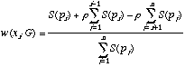 (4)
(4)
where ![]() is a function of the probability of consequence xi; and the weight given up by this branch is
is a function of the probability of consequence xi; and the weight given up by this branch is ![]() , indicating that this branch gives up weight to all branches with consequences lower in value than
, indicating that this branch gives up weight to all branches with consequences lower in value than ![]() , (recall
, (recall
Birnbaum and Chavez (1997) assumed that ![]() ,
,
Research with configural weighting models has shown that one can fit the data fairly well with the simplifying assumption that u(x) = x, for 0 < x < $150. I don't really think that the psychological value of money is proportional to money. I believe that the subjective value of $2 million differs less from $1 million than $1 million differs from $0. I also think that $1 million means less to Bill Gates (who has $billions) than it would to me. But for small amounts of cash (pocket money), the assumption that the value of money is proportional to face value seems reasonable. Also, this approximation makes it easier to interpret and compare parameters.
Subjectively weighted utility (SWU) theory (Edwards, 1954) is the nonconfigural, special case of Equation 1 in which ![]() , so
, so ![]() . Expected utility (EU) theory is the special case of SWU in which
. Expected utility (EU) theory is the special case of SWU in which ![]() ;
; ![]() . Expected value is the special case of EU in which
. Expected value is the special case of EU in which ![]() ;
; ![]() . Although EV and EU theories have been rejected in previous studies (Kahneman & Tversky, 1979; Tversky & Kahneman, 1992; Luce, 1990; Birnbaum, 1999; Birnbaum & Beeghley, 1997; Wu & Gonzalez, 1996), they provide benchmarks for assessing the more complex models, of which they are special cases.
. Although EV and EU theories have been rejected in previous studies (Kahneman & Tversky, 1979; Tversky & Kahneman, 1992; Luce, 1990; Birnbaum, 1999; Birnbaum & Beeghley, 1997; Wu & Gonzalez, 1996), they provide benchmarks for assessing the more complex models, of which they are special cases.
Birnbaum (in press) reported fits of TAX, CPT, EU, and EV models to the data of Internet A and the lab data, to compare the relative accuracy of the models in describing individual data. Each person's data were fit to the models by methods described in Birnbaum and Chavez (1997). After a model was fit to a person's data, it was checked for each choice. The computer program checked if the person indeed picked the gamble with the higher computed utility according to that model and its parameters, and it counted the number of correct predictions (out of 20 choices).
The TAX model was fit with u(x) = x. In Internet A, median estimates of
g and d for the TAX model are .791 and —.333, respectively. This model correctly predicted 15 or more choices (75% correct or better) by 67% of the individuals, including perfect scores for 66 people.The CPT model cannot explain violations of stochastic dominance, event-splitting effects, or violations of cumulative independence. For Internet A, median estimates of
g and c were .743 and .597, respectively. In the Internet sample, 58.5% had 15 or more choices predicted correctly, including 34 with perfect scores. The mean number of choices correctly predicted was significantly higher for the TAX model (15.53) than for CPT (14.91), t(1223) = 8.05*. The TAX model predicted more choices correctly for 614* people; 414 had more predicted correctly by CPT, and 196 were even.For the EU model, utility was estimated as a power function of monetary value, ![]() . For Internet A, median estimate of
. For Internet A, median estimate of
No individual had data that were perfectly consistent with EV. This seemed a bit surprising because a number of people from Internet A with doctorates sent comments that they simply chose the gamble with the higher EV. One person even wrote that anyone who did not choose according to EV (in Internet A) would have to be "insane." However, no one wrote that they actually computed EV, and apparently no one did. For Internet A, EV correctly predicts 15 or more choices for only 16.8% of the judges with a mean of 12.4 correct predictions.
Similar results were obtained in model fits to the lab samples (Birnbaum, in press). In sum, the TAX model is more accurate in predicting choices than CPT, and both of these models are more accurate than EU or EV.
V. DISCUSSION
Systematic violations of stochastic dominance and event-splitting effects are observed in both Internet and lab samples. These phenomena contradict the implications of several models of decision-making, but they are consistent with configural weight theories. Although there are differences between Internet and lab samples, both sets of results would lead to the same conclusions concerning the models. A comparison of fit showed that the configural weight, TAX model fits better than the CPT model that has the same number of estimated parameters. Both of these models fit better than EU, which fit better than EV.
The procedures used in this study differ from those used by Birnbaum and Navarrete (1998), and Birnbaum, et al. (1999). There were fewer trials, a different format for presentation of choices, a computer web form instead of paper and pencil, real financial incentives instead of hypothetical financial incentives, and other differences. Results confirmed previous findings, suggesting that previous results were not fragile with respect to these changes in procedure.
Internet and lab samples yield similar conclusions, indicating that the findings are not unique to college students, tested in laboratories. Internet B replicates the findings of other investigators with variations of the Allais paradoxes (Allais & Hagen, 1979; Wu & Gonzalez, 1996), showing that these paradoxes can be replicated with smaller cash consequences and real incentives.
These studies demonstrate the feasibility of using the Internet to check results with a large, diverse sample. Compared to my usual research, which typically takes six months to collect data for 100 college students, it was quite pleasant to collect 1224 sets of data in four months and 737 in the next 5 weeks. It may not always be as easy as it was in 1998 to recruit participants on the web. As more people put their experiments on the web, there may develop more competition for people willing to take part in tests and experiments. On the other hand, more and more people surf the net each day, so it is difficult to forecast whether the number of experiments or the number of willing participants will grow at a faster rate.
Internet research has two potential problems that are obvious to those who venture there: sampling and control. With lab studies, one can control the conditions. For example, we can ensure that laboratory subjects do not use calculators to compute expected value. Alternately, we could require them to do so. With an Internet study, we have very little control over the conditions. In these studies, there were no instructions one way or the other concerning the use of calculators. When people began sending me email that they thought everyone would just choose the gamble with the higher EV, I wondered if perhaps I should have given an instruction concerning calculators. But that very instruction might have given the idea to people, who might otherwise not have thought of it. And if I gave such an instruction, how would I know for certain if it was followed?
We could ask people to follow instructions, and we could ask them if they did. One might hope that variations of conditions would simply introduce random error that would average out with large samples. Ultimately, we must rely on the subject's honesty, on indirect checks, or the hope that deviations of protocol don't matter to the case at hand. In this study, it seems unlikely that people used calculators because not even one person was perfectly consistent with EV. But this issue illustrates one of many possible aspects of control that would not be issues in lab experiments.
I think it would be an oversimplification to talk of the university subject pool and Internet as if they referred to two populations. I don't think that the Internet is really a single population, but instead may be regarded as many different sub-populations tangled together. Nor are the samples found by these methods going to be constant over time. The Internet is ever changing, and as equipment becomes cheaper and easier to use, we can expect changes in the landscape and the travelers on this highway. In the past few years, the percentage of females on the Internet has increased sharply. Notice that both Internet A and B samples have more females than males. Subject pools have also changed over time, as a greater percentage of the general population enrolls in college and as an even greater percentage of females have elected to attend college and to enroll in psychology.
Slight changes in methods used to recruit participants in an experiment could potentially have great effects. This study used methods intended to reach a highly educated population, especially in the field of decision making. The fact that 95 with doctorates were recruited who have read a scholarly work on decision making suggests that the method of recruitment succeeded in reaching its target audience.
Although one can use methods intended to reach certain groups, Internet experimenters do not have complete control of recruitment. For example, in an Internet study of sexual behavior, an Abuse web-site cross-listed the sex survey reported in Bailey, Foote, & Throckmorton (this volume). This placing of a "link" by another well-meaning person recruited many people with histories of abuse to the sexual survey. If the purpose of the survey had been to estimate prevalence of abuse in the population, this link placed by another person might have altered the conclusions.
If demographic or other individual difference variables affect the behavior in question, then one can measure these and study their correlations with the results. The Internet certainly affords greater opportunities for recruiting a very heterogeneous sample. In the studies reviewed here, the Internet samples were much more diverse with respect to age and education than the sample recruited from the subject pool. Rates of violation of stochastic dominance were correlated with gender, education, and experience reading a scholarly work on decision making. The Internet sample was less likely to violate stochastic dominance than the lab sample, and the Internet sample also differed from the lab sample by having a lower percentage of females, more education, greater age, and more likely to have read a paper on decision making. Thus, the difference between Internet and lab results appears to be what one would expect from the demographic differences between the groups.
Education, which correlated with incidence of violations of stochastic dominance, is probably also correlated with variables not measured that might be causal agents. For example, those with more education are probably also higher in intelligence and wealth than those with less education. Therefore, lower incidence of stochastic dominance by the highly educated might be due to higher intelligence, for example, rather than to the effects of education per se. Experiments with random assignment to different types of education could determine if specific training would reduce violations of stochastic dominance.
In sum, Internet research confirms phenomena that violate the RSDU/RDU/CPT theories of decision making. Results are more compatible with Birnbaum's (1999) configural weight TAX model, which implies systematic violations of stochastic dominance and event splitting effects. At the same time, Internet data reveal correlations between these violations and demographic variables. In this case, Internet data both reinforced the results of laboratory research and also revealed variables that may moderate the generalization from lab research with undergraduates to research with other populations.
REFERENCES
Allais, M., & Hagen, O. (Ed.). (1979). Expected utility hypothesis and the Allais paradox. Dordrecht, The Netherlands: Reidel.
Becker, J., & Sarin, R. (1987). Lottery dependent utility. Management Science, 33, 1367-1382.
Birnbaum, M. H. (1974). The nonadditivity of personality impressions. Journal of Experimental Psychology, 102, 543-561.
Birnbaum, M. H. (1997). Violations of monotonicity in judgment and decision making. In A. A. J. Marley (Ed.), Choice, decision, and measurement: Essays in honor of R. Duncan Luce (pp. 73-100). Mahwah, NJ: Erlbaum.
Birnbaum, M. H. (1999). Paradoxes of Allais, stochastic dominance, and decision weights. In J. Shanteau, B. A. Mellers, & D. A. Schum (Eds.), Decision science and technology: Reflections on the contributions of Ward Edwards (pp. 27-52). Norwell, MA: Kluwer Academic Publishers.
Birnbaum, M. H. (in press). Testing critical properties of decision making on the Internet. Psychological Science, in press.
Birnbaum, M. H., & Beeghley, D. (1997). Violations of branch independence in judgments of the value of gambles. Psychological Science, 8, 87-94.
Birnbaum, M. H., & Chavez, A. (1997). Tests of theories of decision making: Violations of branch independence and distribution independence. Organizational Behavior and Human Decision Processes, 71(2), 161-194.
Birnbaum, M. H., & Martin, T. (submitted). Violations of stochastic dominance and event-splitting effects by financially motivated decision makers. submitted for publication, 00, 000-000.
Birnbaum, M. H., & McIntosh, W. R. (1996). Violations of branch independence in choices between gambles. Organizational Behavior and Human Decision Processes, 67, 91-110.
Birnbaum, M. H., & Navarrete, J. (1998). Testing descriptive utility theories: Violations of stochastic dominance and cumulative independence. Journal of Risk and Uncertainty, 17, 49-78.
Birnbaum, M. H., Patton, J. N., & Lott, M. K. (1999). Evidence against rank-dependent utility theories: Violations of cumulative independence, interval independence, stochastic dominance, and transitivity. Organizational Behavior and Human Decision Processes, 77, 44-83.
Birnbaum, M. H., & Stegner, S. E. (1979). Source credibility in social judgment: Bias, expertise, and the judge's point of view. Journal of Personality and Social Psychology, 37, 48-74.
Humphrey, S. J. (1995). Regret aversion or event-splitting effects? More evidence under risk and uncertainty. Journal of risk and uncertainty, 11, 263-274.
Kahneman, D., & Tversky, A. (1979). Prospect theory: An analysis of decision under risk. Econometrica, 47, 263-291.
Luce, R. D. (1998). Coalescing, event commutativity, and theories of utility. Journal of Risk and Uncertainty, 16, 87-113.
Luce, R. D. (1990). Rational versus plausible accounting equivalences in preference judgments. Psychological Science, 1, 225-234.
Luce, R. D., & Fishburn, P. C. (1991). Rank- and sign-dependent linear utility models for finite first order gambles. Journal of Risk and Uncertainty, 4, 29-59.
Luce, R. D., & Fishburn, P. C. (1995). A note on deriving rank-dependent utility using additive joint receipts. Journal of Risk and Uncertainty, 11, 5-16.
Machina, M. J. (1982). Expected utility analysis without the independence axiom. Econometrica, 50, 277-323.
Quiggin, J. (1982). A theory of anticipated utility. Journal of Economic Behavior and Organization, 3, 324-345.
Quiggin, J. (1985). Subjective utility, anticipated utility, and the Allais paradox. Organizational Behavior and Human Decision Processes, 35, 94-101.
Quiggin, J. (1993). Generalized expected utility theory: The rank-dependent model. Boston: Kluwer.
Starmer, C., & Sugden, R. (1993). Testing for juxtaposition and event-splitting effects. Journal of Risk and Uncertainty, 6, 235-254.
Tversky, A., & Kahneman, D. (1992). Advances in prospect theory: Cumulative representation of uncertainty. Journal of Risk and Uncertainty, 5, 297-323.
Tversky, A., & Wakker, P. (1995). Risk attitudes and decision weights. Econometrica, 63, 1255-1280.
von Winterfeldt, D. (1997). Empirical tests of Luce's rank- and sign-dependent utility theory. In A. A. J. Marley (Ed.), Choice, decision, and measurement: Essays in honor of R. Duncan Luce (pp. 25-44). Mahwah, NJ: Erlbaum.
Wakker, P., & Tversky, A. (1993). An axiomatization of cumulative prospect theory. Journal of Risk and Uncertainty, 7, 147-176.
Weber, E. U. (1994). From subjective probabilities to decision weights: The effects of asymmetric loss functions on the evaluation of uncertain outcomes and events. Psychological Bulletin, 114, 228-242.
Wu, G., & Gonzalez, R. (1996). Curvature of the probability weighting function. Management Science, 42, 1676-1690.
Table 1. Choices used to test stochastic dominance and other properties, common to all three samples.
|
Choice Type No. |
Choice |
% Choice Internet A B Lab |
|||
|
1 |
A: .50 to win $0 B: .50 to win $25 .50 to win $100 .50 to win $35 |
48 |
52 |
58 |
|
|
2 |
C: .50 to win $0 D: .50 to win $45 .50 to win $100 .50 to win $50 |
60 |
63 |
69 |
|
|
3 |
E: .50 to win $4 F: .50 to win $4 .30 to win $96 .30 to win $12 .20 to win $100 .20 to win $100 |
6 |
9 |
8 |
|
|
4 |
G: .40 to win $2 H: .40 to win $2 .50 to win $12 .50 to win $96 .10 to win $108 .10 to win $108 |
96 |
97 |
94 |
|
|
5 |
G + G— |
I: .05 to win $12 J: .10 to win $12 .05 to win $14 .05 to win $90 .90 to win $96 .85 to win $96 |
58 |
64 |
73 |
|
7 |
G — G+ |
M: .06 to win $6 N: .03 to win $6 .03 to win $96 .03 to win $8 .91 to win $99 .94 to win $99 |
54 |
46 |
36 |
|
11 |
GS + GS— |
U: .05 to win $12 V: .05 to win $12 .05 to win $14 .05 to win $12 .05 to win $96 .05 to win $90 .85 to win $96 .85 to win $96 |
10 |
14 |
15 |
|
13 |
GS — GS+ |
Y: .03 to win $6 Z: .03 to win $6 .03 to win $6 .03 to win $8 .03 to win $96 .03 to win $99 .91 to win $99 .91 to win $99 |
95 |
95 |
92 |
Note: Choice types are described in the introduction. Percentages show choices for the gamble printed on the right in the table.  Choices 1 and 2 assess risk aversion; Choices 3 and 4 test consequence monotonicity ("transparent" dominance).


Table 2.  Demographic Characteristics of the Samples (Percentages).
Characteristic |
Internet A (n = 1224) |
Internet B (n = 737) |
Lab (n = 124) |
Age is 22 years and under |
20 |
22 |
91 |
Older than 40 years |
20 |
24 |
0 |
College graduate |
60 |
47 |
0 |
Doctorates |
11 |
3 |
0 |
Read scientific paper on decision making |
31 |
19 |
13 |
Female |
56 |
61 |
73 |
Violations of stochastic dominance |
52 |
59 |
68 |
Violations of consequence monotonicity |
7 |
8 |
11 |
Note: Violations of stochastic dominance and consequence monotonicity are averaged over Choices 5 and 7 and Choices 11 and 13, respectively.


Table 3. Violations of stochastic dominance and event-splitting effects in Internet B (n=737) and Lab samples (n = 124, two replicates), respectively.
Internet Sample B |
Lab Sample |
|||||||
Choice 11 |
Choice 11 |
|||||||
Choice 5 |
GS+ |
GS— |
Choice 5 |
GS+ |
GS— |
|||
G+ |
31.5 |
4.5 |
36.0 |
G+ |
21.8 |
4.8 |
26.6 |
|
G— |
54.3* |
9.2 |
63.5 |
G— |
62.5* |
9.7 |
72.2 |
|
86.0 |
10.5 |
84.3 |
14.5 |
|||||
Choice 13 |
Choice 13 |
|||||||
Choice 7 |
GS+ |
GS— |
Choice 7 |
GS+ |
GS— |
|||
G+ |
43.3 |
2.6 |
54.0 |
G+ |
33.1 |
2.8 |
35.9 |
|
G— |
51.2* |
2.6 |
54.0 |
G— |
58.5* |
5.6 |
64.1 |
|
94.6 |
5.2 |
91.6 |
8.4 |
|||||
Note: percentages sum to less than 100, due to a few who did not respond to all items.

Table 4. Violations of stochastic dominance and monotonicity related to gender and education in Internet Samples A, B, and lab sample.
Sex |
Education (years) |
Stochastic Dominance (%)
G—
f G+ A B Lab |
Monotonicity (%)
GS—
f GS+ A B Lab |
Number of Subjects A B Lab |
||||||
F |
< 16 |
60.2 |
66.1 |
70.4 |
9.6 |
11.3 |
11.8 |
318 |
248 |
91 |
F |
16 |
61.9 |
56.8 |
10.0 |
8.1 |
206 |
148 |
0 |
||
F |
17-19 |
44.9 |
58.5 |
7.4 |
13.4 |
108 |
41 |
0 |
||
F |
20 |
41.7 |
54.5 |
1.9 |
9.1 |
54 |
11 |
0 |
||
M |
< 16 |
53.1 |
56.0 |
62.9 |
6.4 |
7.8 |
10.6 |
163 |
141 |
33 |
M |
16 |
42.6 |
55.6 |
6.4 |
10.2 |
195 |
98 |
0 |
||
M |
17-19 |
36.4 |
56.3 |
2.3 |
3.1 |
88 |
32 |
0 |
||
M |
20 |
37.5 |
57.1 |
6.2 |
7.1 |
80 |
14 |
0 |
||
Notes: Education < 16 indicates less than bachelor's degree; 16= Bachelor's degree; 17-19 = Postgraduate studies; 20 = doctorate. Percentages indicate percentage of violations of stochastic dominance and consequence monotonicity, averaged over two choices.
Table 5. Choices used to test Allais common ratio and common consequence paradoxes in Internet B.
|
Choice Choice No. Type |
Choice |
% Choice Internet B (n = 737) |
|
|
9 |
S R |
Q: .75 to win $0 R: .80 to win $0 .25 to win $60 .20 to win $80
|
43 |
|
16 |
S 4 R4 |
e: $60 for sure f: .20 to win $0 .80 to win $80
|
10 |
|
15 |
S * R* |
c: .85 to win $0 d: .90 to win $0 .15 to win $40 .10 to win $100
|
70 |
|
18 |
S *+C R*+C |
i: $40 for sure j: .05 to win $0 .85 to win $40 .10 to win $100 |
50 |
|
14 |
R ' S' |
a: .95 to win $0 b: .93 to win $0 .05 to win $96 .07 to win $80
|
61 |
|
17 |
R '+C1 S'+C1 |
g: .45 to win $0 h: .43 to win $0 .50 to win $80 .57 to win $80 .05 to win $96 |
44 |
|
8 |
R '+C2 S'+C2 |
O: .07 to win $0 P: .05 to win $0 .88 to win $80 .95 to win $80 .05 to win $96 |
60 |
|
19 |
R '+C3 S'+C4 |
k: .02 to win $0 l: $80 for sure .93 to win $80 .05 to win $96 |
70 |
Note: Percentages show preferences for the gamble printed on the right in the table.


APPENDIX: ADDITIONAL DETAILS OF EXPERIMENT
This appendix gives more detail on the HTML page and recruitment methods. The web site was announced by an email message sent to all members of the Society for Judgment and Decision-Making and Society for Mathematical Psychology.  It was suggested to major search engines, announced in web sites that list contests and games with prizes, and described by Meta tags within in the web page (these help search engines locate the page).  Links to the site were established (among others) in the American Psychological Society's list of on-line experiments, maintained by John Krantz, the European Web Lab, maintained by Ulf Reips, and John Baron's lab site (see chapters by Baron, Krantz & Dalal, and Reips).
	The HTML below shows the key features of the web page to conduct an experiment on choices between gambles.  Portions of the instructions and many of the trials are omitted, leaving the parts essential to explaining how the page works.  Every HTML page has the
<HTML> and </HTML> tags, which identify the begining and end of the page. Material between the <HEAD> and </HEAD> contains the head of the page, and the <BODY> </BODY> tags identify the begining and end of the body of the page. In the head are the TITLE and META tags. Some search engines use the content in META tags to find keywords and descriptions of the pages. The TITLE appears at the top of the page in the browser's display of the page. The <H3></H3> tags identify a size 3 heading, which is fairly large. <P> tags identify paragraphs, and unlike most tags, do not require a closing </P> tag. The <FORM> tag identifies the next material as a form, and shows where the data will be sent when the user pushes the "submit" button. The ACTION of a form sends the data to a URL that contains a script that was created by PolyForm [http://polyform.ora.com], a program that makes a script to decode and organize the data, place them in a file, and send the browser to a page where they read a thank-you message. The URL listed below refers to a real script, but not the one actually used in the study. Each variable name is preceded by a sequential number from 00 to 29, which determines the order by which PolyForm's script will organize the data in the data file. The </FORM> tag signals the end of the form. The first two variables created by <INPUT TYPE="hidden" ...> are hidden variables, the date and time, available from PolyForm script. They are "hidden" because they are not displayed in the page, but they are placed into the data file. These variables uniquely identify each data record, and it can be helpful to be able to look up a participant's record by time and date. The <PRE> and </PRE> tags instruct the browser to display everything between those tags in "preformatted text." Browsers typically use an equally spaced font (like courier) to display preformatted text. Line returns, tabs, etc. are preserved in preformatted text. In this case, I chose preformatted text to make it easy to make all of the trials uniform in appearance without having to use tables or other tricks to align the text. The line that reads, <input type="text" name="02Name" size=60 maxlength=60> Illustrates use of text type input. This tag creates a text box that is 60 characters wide, where the person was instructed to type his or her email address. If the maxlength had been bigger than 60, then someone could have continued to type after 60 columns until the maximum was reached. I think it is often best to make the size and maxlength equal, so the person has an idea of how much space is available for their comment, or whatever. Sometimes, you might want to allow a little extra room, for the last few words. In the age box, I allowed an extra digit, because if anyone over 100 participated, I would certainly want to know about it. After a person types in his or her email address in this box, that typing will appear in the data file as the third variable, after date and time. (Sometimes, if a person types in commas, it may create problems for data analysis later. A comma stripping routine is included in the study by Bailey, et al in this volume.) The request for age also uses the same method, as does the input field for education, and later in the form, the text box for comments. The key to this study is the use of the radio buttons. The properties of radio buttons seem perfectly suited for choice experiments. The question about sex (male or female) uses radio buttons, as do the main 20 choices in the experiment. (I have edited out most of the questions below, and also removed most of the instructions). Each button requires its own <INPUT TYPE="radio" ...> tag. Notice that for the sex question, there are three tags, all with the same NAME. There is only one selected (blackened) dot for each set of radio buttons, which are defined (connected) by the same NAME. Thus, clicking one of the empty buttons darkens that button (selects it), and simultaneously deselects the previously selected button. Although one could request sex with two radio buttons (no pun intended), I strongly advise against it. The reason I use three radio buttons for gender and for decision problems is as follows: with only two choices, one will be selected before the person responds. That way, everyone (both you and the subject) may become confused whether the subject selected that choice, or if perhaps it was that way to start. When we request choices between gambles, if one choice is selected in advance, the subject may be reluctant to switch to the other choice, or may forget that she didn't select that choice. For these reasons, I use three radio buttons for each 2-alternative choice. Note that the "nothing" button is preselected. This button is placed before the trial number, in the left margin. These buttons in the margin serve two purposes. First, they keep track of nonresponse, and second, they make it easy for the participant to see if each trial has been completed. Note that the nonresponse is assigned the value "0". It could also have been assigned a null value, "". However, I thought ahead to data analysis, and it occurred to me that a blank field of data might get lost if this file were saved as formatted text and then imported to a statistics program, using freefield. Because the values of male and female are assigned M and F, a "0" is clearly a nonresponse, so there is no confusion when it is time to analyze the data, and it holds the place of the variable. Each of the choices in the decision experiment was handled in the same way. I used 3 radio buttons for each choice, with the third button holding the nonresponse. A person can scroll down the list of questions, and note if any of the buttons in the left margin are still filled. Nonresponse was assigned the value 0, choice on the left was -1, and choice of the right was assigned the value 1. This numerical assignment means that the mean of this variable will indicate if the majority chose the gamble on the left or right. The last items are of types already discussed. The last "hidden" variable allows me to make note of when conditions have changed (I can change to Exp2a, Exp2b, Exp3a, etc. ) and it also provides a variable that is easy to align during data analysis. When the data have been read into Excel or SPSS, if the last variable is not "exp2b," then something is amiss in the importing of the data. The <INPUT TYPE="submit" VALUE="I'm finished"> creates a button with the words "I'm finished" printed on it. When the subject pushes this button, the data are sent to the script to be placed in the data file, and the subject sees a thank you message on the screen. If you would like to check how the page works, and see sample data, you can first go to URL http://psych.fullerton.edu/mbirnbaum/exp2a.htm Then, when you have completed the experiment, use your FTP program to download the following file: data.csv. You need the following to reach the FTP site, which only supports downloading. Host: psych.fullerton.edu User ID: guest Password: guest99 Directory: (you should leave this blank). The file, data.csv, will contain your data, including the time and date that you participated. You are welcome to use the generic script, to try out these principles, which will send data to this file, from which you can retrieve your data by FTP. Your HTML page can be on diskette, which you can load directly into your browser, or it can be on your local server. As long as you use the script address shown, the data will go to this data file. The file, data.csv, will be erased from time to time when it gets large, so you should not leave anything there of any value. Also, since that file will be public to all who read this paper, I advise you not to put anything personal or sensitive there, since many people may read that file. In the long run, you will need to get access to a server and put your own scripts in place to allow you to collect data on your own computer. You can also change the ACTION in the FORM tag to read ACTION="mailto:user@address.ext", where user@address.ext is your email address. That method can get you data by email, which allows you to check an experiment, but is not practical for large projects. Table 6. HTML (abbreviated) for the decision experiment. <HTML> <HEAD> <META NAME="keywords" CONTENT="Gamble, decision making, experiment, science, win money"> <META NAME="description" CONTENT="Choose between gambles, without risk, and help science by participating as a subject in decision making experiment. You might win money."> <TITLE>Decision Experiment</TITLE> </HEAD> <BODY> <H3>Decision-Making Experiment: Choices between Gambles</H3> <P>This is a study of decision making ...Decide first if you want to participate. You must be over 18, and each person can participate only once. Scroll down and look over the questionnaire. It usually takes about 10 minutes. Also note: Study ends and prizes awarded 9/15/98.<P> <FORM METHOD="POST" ACTION="http://psych.fullerton.edu/cgi-win/polyform.exe/generic"> <input type="hidden" name="00Date" value="pfDate"> <input type="hidden" name="01Time" value="pfTime"> <PRE> Email address:<input type="text" name="02Name" size=60 maxlength=60> We will notify you by email if you are a winner. Country:<INPUT TYPE=TEXT NAME=03Con SIZE=20 maxlength=25> Age:<INPUT TYPE=TEXT NAME=04Age SIZE=2 maxlength=3> You must be over 18 years to participate. <input type="radio" name="05sex" value="0" checked>Are you Male or Female? <input type="radio" name="05sex" value="F">Female OR <input type="radio" name="05sex" value="M">Male Education (in years). If you are a college graduate, put 16. If you have a Ph.D., put 20. Education: <INPUT TYPE=TEXT NAME=06Ed SIZE=2 maxlength=2> Years. Now, look at the first choice, No. 1, below... Think of probability as the number of tickets in a bag containing 100 tickets, divided by 100. Gamble A has 50 tickets that say $100 and 50 that say $0, so the probability to win $100 is .50 and the probability to get $0 is .50. ...(more instructions were here) <input type="radio" name="07v1" value="0" checked>1. Which do you choose? <input type="radio" name="07v1" value="-1">A: .50 probability to win $0 .50 probability to win $100 OR <input type="radio" name="07v1" value="1">B: .50 probability to win $25 .50 probability to win $35 <input type="radio" name="08v2" value="0" checked>2. Which do you choose? <input type="radio" name="08v2" value="-1">C: .50 probability to win $0 .50 probability to win $100 OR <input type="radio" name="08v2" value="1">D: .50 probability to win $35 .50 probability to win $45 ...(more trials were here).... ----------- <input type="radio" name="27v21" value="0" checked>21. Have you ever read a scientific paper (i.e., a journal article or book) on the theory of decision making or on the psychology of decision making? <input type="radio" name="27v21" value="No">No. Never. OR <input type="radio" name="27v21" value="Yes">Yes, I have. <P> COMMENTS:<INPUT TYPE="text" NAME="28COMS" size=65 maxlength=65> Please check to make sure that you have answered all of the Questions. <input type="hidden" name="29Exp2" value="exp2b"> When you are finished, push this button to send your data: <INPUT TYPE="submit" VALUE="I'm finished."> </PRE></FORM></BODY></HTML>